


Popular Imagery of Money on the MoveFor most financial commentators an important factor that either reinforces or weakens the effect of changes in the money supply on economic activity and prices is the “velocity of money”. An image from an article on the intertubes that “explains” the velocity of money (one of the articles we came across started out as follows: “The economy runs smoothly only when there is enough money in circulation. How much is enough?” The effect reading this has on us is not unlike that produced by the sound of fingernails scraping a chalkboard). We have found that many people find it extremely difficult to wrap their mind around the fact that the velocity concept actually doesn’t make sense, and that the matter has to be viewed from a different perspective. As an aside, we have noticed in discussions that even those who do eventually accept that a different conceptual approach is required, often insist on continuing to use the term because it “doesn’t matter what we call it”, or “to keep things simple” and similar excuses. It makes one feel like a priest trying to exorcise a particularly stubborn demon. It is alleged that when the velocity of money rises, all other thing being equal, the buying power of money declines (i.e., the prices of goods and services rise). The opposite occurs when velocity declines. If, for example, it was found that the quantity of money had increased by 10% in a given year, — while the price level as measured by the consumer price index has remained unchanged — it would mean that the velocity of circulation must have slowed by about 10%. |
 Illustration via supplychainbigairo.blogspot.com - Click to enlarge |
The Mainstream View of Money Velocity
|
Velocity of M1 Money Stock, 1960 - 2017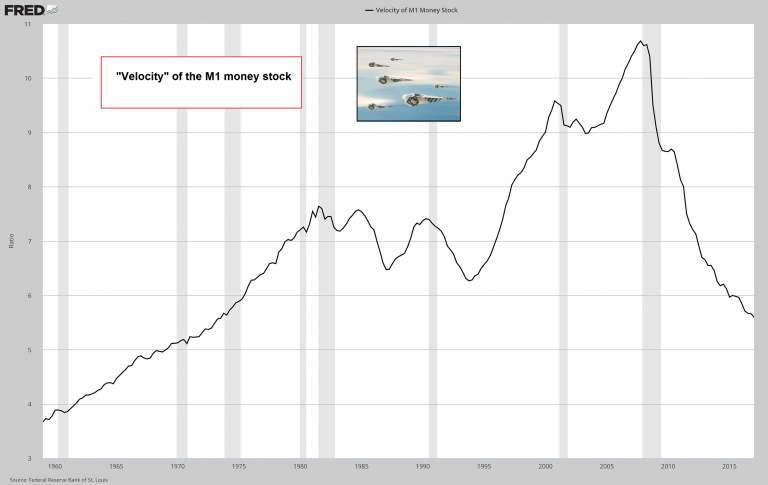 - Click to enlarge |
A $10 bill, which is circulating with a velocity of ‘3’ financed $30 worth of transactions in that year. Consequently, if there are $3000 billion worth of transactions in an economy during a particular year and there is an average money stock of $500 billion during that year, then each dollar of money is used on average 6 times during the year (since 6*$500 billion =$3000).
The $500 billion of money is boosted by means of a velocity factor to become effectively $3000 billion. From this it is established that
Velocity = Value of transactions / supply of money
This expression can be summarized as
V = P*T/M
Where V stands for velocity, P stands for average prices, T stands for volume of transactions and M stands for the supply of money. This expression can be further rearranged by multiplying both sides of the equation by M. This in turn will give the famous equation of exchange
M*V = P*T
This equation states that money times velocity equals value of transactions. Many economists employ GDP instead of P*T thereby concluding that
M*V = GDP = P*(real GDP)
The equation of exchange appears to offer a wealth of information regarding the state of the economy. For instance, if one were to assume a stable velocity, then for a given stock of money one can establish the value of GDP. Furthermore, information regarding the average price or the price level allows economists to establish the state of real output and its rate of growth.
| Most economists take the equation of exchange very seriously. The debates that economists have are predominantly with respect to the stability of velocity. Thus if velocity is stable then money becomes a very powerful tool in tracking the economy.
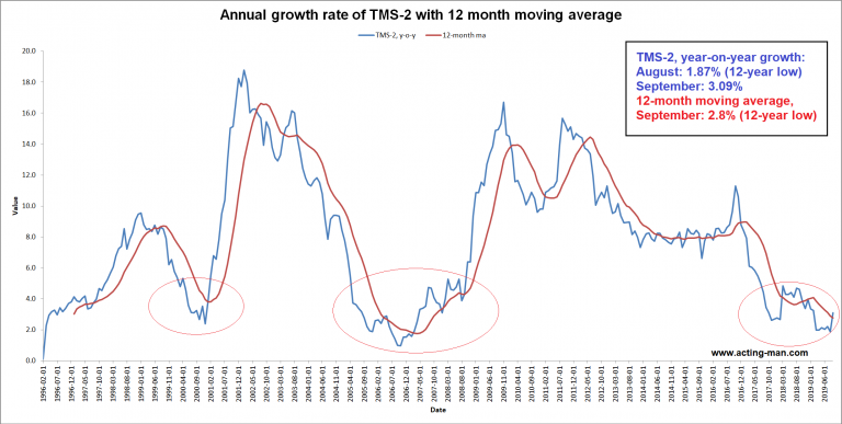
The importance of money as an economic indicator however diminishes once velocity becomes less stable and hence less predictable. It is held an unstable velocity implies an unstable demand for money, which makes it so much harder for the central bank to navigate the economy along the path of economic stability. Now consider this chart, which depicts the broad US true money supply TMS-2 (black line), nominal GDP (red line) – both indexed – and the “velocity” of M1 (the formula is simply [nominal GDP/money stock]). What does this really tell us? Consider in particular the time period within the blue rectangle (which coincides with the sharp decline in “V”), and compare it to the preceding era. The trends within the rectangle essentially tell us “the Fed printed a lot of money, which did not translate into equivalent GDP growth”. Well… duh (if it had, we would actually not have experienced a lot of growth, but a runaway surge in consumer prices – remember that nominal GDP is employed in the calculation). Moreover, prior to the GFC, when the creation of additional money was largely accomplished by fractionally reserved banks expanding credit, GDP growth merely tracked the pace of monetary inflation (this fact is actually worth a separate article). What can not be concluded from this chart is that “velocity” has any meaning besides being a fudge factor in the tautological “equation of exchange”. In short, the empirical data appear to be in line with what economic logic already tells us. Obviously, the demand for money (i.e., the demand for holding cash balances) will be a major driver affecting the purchasing power of money, ceteris paribus. Since society as a whole cannot lower its cash balances (someone always has to hold the existing money stock), a decline in the demand for money will simply result in a decline of its purchasing power. When people lose confidence in government-issued money – which usually happens after its supply has increased at an uncommon pace for a considerable time period and a sufficiently large number of people abandons the belief that the expansion will ever stop – this may well show up in “velocity” charts, particularly in the final stage of an inflationary process, when the monetary system begins to break down (currently observable in Venezuela). This will mainly indicate that a “flight into real values” has commenced and that the collapse in purchasing power is beginning to exceed the speed at which new money is printed. This is a typical feature of such end games – concurrently with deep contractions in real economic output. The main point is that the associated surge in “velocity” would be a symptom, not a cause. |
TMS - 2, Nominal US GDP and Velocity of M1, 1988 - 2017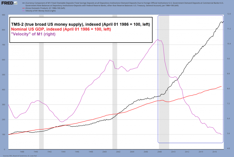 - Click to enlarge |
Why Velocity has Nothing to do With the Purchasing Power of Money
But does velocity have anything to do with the prices of goods? Prices are the outcome of individuals’ purposeful actions. Thus John the baker believes that he will raise his living standard by exchanging ten loaves of bread for $10, which will enable him to purchase five kg of potatoes from Bob the potato farmer. Likewise, Bob has concluded that by means of $10 he will be able to secure the purchase of ten kg of sugar, which he believes will raise his living standard.
By entering an exchange, both John and Bob are able to realize their goals and thus promote their respective well-being. John has agreed that it is a good deal to exchange 10 loaves of bread for $10 for it will enable him to procure 5kg of potatoes. Likewise Bob has concluded that $10 for his 5kg of potatoes is a good price for it will enable him to secure 10kg of sugar. Observe that price is the outcome of different ends, and hence the different importance that both parties to a trade assign to means.
It is the purposeful actions of individuals that determine the prices of goods, not some mythical velocity. Indeed, according to Ludwig von Mises, the whole concept of velocity is hollow. As he writes in Human Action:
In analyzing the equation of exchange one assumes that one of its elements — total supply of money, volume of trade, velocity of circulation — changes, without asking how such changes occur. It is not recognized that changes in these magnitudes do not emerge in the Volkswirtschaft [ed note: political economy, or more loosely ‘economy’] as such, but in the individual actors’ conditions, and that it is the interplay of the reactions of these actors that results in alterations of the price structure. The mathematical economists refuse to start from the various individuals’ demand for and supply of money. They introduce instead the spurious notion of velocity of circulation, fashioned according to the patterns of mechanics.
Furthermore, money never circulates as such:
Money can be in the process of transportation, it can travel in trains, ships, or planes from one place to another. But it is in this case, too, always subject to somebody’s control, is somebody’s property.
| Ludwig von Mises reminds us that changes in “macroeconomic magnitudes” result from the purposeful actions of human beings with their own volition and goals. The economy is definitely not a machine.
Consequently, the fact that so-called velocity is ‘3’ or any other number has nothing to do with average prices and the average purchasing power of money as such. Moreover, the average purchasing power of money cannot even be established. For instance, in a transaction the price of one dollar was established as one loaf of bread. In another transaction the price of one dollar was established as 0.5kg of potatoes, while in the third transaction the price is one kg of sugar. Observe that since bread, potatoes and sugar are not commensurable, no average price of money can be established. Now, if the average price of money can’t be established it means that the average price of goods can’t be established either. Consequently, the entire equation of exchange falls apart. Conceptually the whole thing is not a tenable proposition and covering a fallacy in mathematical clothing cannot make it less fallacious. |
 - Click to enlarge |
| According to Rothbard, in Man, Economy, and State:
Even if we were to accept that the essential service of money is its speed of circulation, there is no way that this characteristic of money could explain the purchasing power of money. On this Mises explains in Human Action:
|
TMS - 2 and Nominal GDP, 1986 - 2017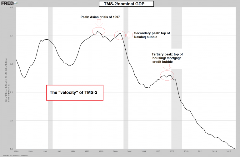 - Click to enlarge |
Full story here Are you the author?
Tags: central banks,newslettersent,On Economy


1 comments
Spencer
2017-11-12 at 19:08 (UTC 2) Link to this comment
If money velocity doesn’t matter, then how did N-gNp hit 20.1% in the first qtr. of 1981?