


George Dorgan
My articles My siteAbout meMy videosMy books
Follow on:LinkedINTwitterSeeking Alpha
CFA SocietyEconomicBlogs
Mainstream Economic Theory: The Medium Run
The medium run is a notion introduced by Blanchard in his book on macroeconomics. The aim of this page is to provide economic theory and criteria for the medium run. We concentrate on main-stream economics or “New Consus Macroeconomics” as defined here, but compare its theories with post-keynesians. The following completely new edition best represents the mainstream:

Check here to see more details.
In the following we will represent axioms valid in the medium run for the neoclassical mainstream:
The AS-AD model
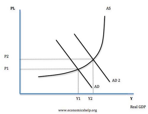
The main mode is the AD-AS model and the main variable for the medium is the aggregate demand.
Economic growth is an increase in real GDP. It means an increase in the value of goods and services produced in an economy. The rate of economic growth measures the annual percentage increase in real GDP. There are several factors affecting economic growth, but it is helpful to split them up into:
Demand-Side Factors Influence Growth of Aggregate Demand (AD)
AD= C+I+G+X-M
Therefore a rise in Consumption, Investment, Government spending or exports can lead to higher AD and higher economic growth.
Graph Showing Rise in AD
What Could Affect AD?
Interest Rates. Lower interest rates would make borrowing cheaper and should encourage firms to invest and consumers to spend. People with mortgages will have lower monthly mortgage payments so more disposable income to spend. However, recently we had a period of zero interest rates, but due to low confidence and reluctant banks growth was still sluggish.
Consumer Confidence. Consumer and business confidence is very important for determining economic growth. If consumers are confident about the future they will be encouraged to borrow and spend. If they are pessimistic they will save and reduce spending.
Asset Prices. Rising house prices create a positive wealth effect. People can remortgage against the rising value of their home and this encourages more consumer spending. House prices are an important factor in the UK, because so many people are homeowners.
Real Wages. Recently, the UK has experienced a situation of falling real wages. Inflation has been higher than nominal wage, causing a decline in real incomes. In this situation, consumers will have to cut back on spending reducing their purchase of luxury items.
Value of Exchange Rate. If a currency devalued, exports would become more competitive and imports more expensive. This would help to increase demand for domestic goods and services. A depreciation could cause inflation, but in the short term at least it can provide a boost to growth.
Banking Sector. The 2008 Credit crunch showed how influential the banking sector can be in determining investment and growth. If the banks lose money and no longer want to lend, it can make it very difficult for firms and consumers leading to a decline in investment.
Monetary and Fiscal Policy may affect monetary and fiscal policy
Unfortunately the model is unsound. If you dig into it you find contradictions that can’t be papered over. One example is that the AS curve depends on the idea that input prices for firms systematically lag output prices, but do you really want to argue the theoretical and empirical case for this? Or try the AD assumption that, even as the price level and real output in the economy go up or down, the money supply remains fixed. (via Peter Dorman)
The Labor market, growth and inflation
Simple production function: Y = N, for N is employment
- How costly it would be for the firm to replace him—the nature of the job.
- How hard it would be for him to find another job—labor market conditions.
It depends on three factors:
- The expected price level,
- The unemployment rate, u
- A catchall variable, z, that catches all other variables that may affect the outcome of wage setting.
Price and Wage Determination
Firms set their price according to
P = (1 + m) W
The term m is the markup of the price over the cost of production. If all markets were perfectly competitive, m = 0, and P = W (one production factor only in this model).
Natural rate of unemployment
If we assume that P = then we obtain the wage-setting relation:
and the price-setting relation:
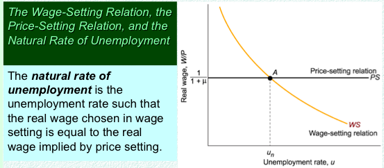
Natural Rate of Unemployment - Click to enlarge
An increase of unemployment benefits leads to a higher natural rate of unemployment.
A higher markup decreases real wages and leads to a higher natural rate of unemployment.
Unemployment and growth: Okun’s law
In part, economists care about a nation’s output (or, more specifically, its Gross Domestic Product) because output is related to employment, and one important measure of a nation’s well-being is whether those people who want to work can actually get jobs.Therefore, it’s important to understand the relationship between output and the unemployment rate. The (approximate) relationship between output and unemployment is referred to as Okun’s Law, after economist Arthur Okun who originally developed the concept in 1962.When an economy is at its “normal” or long-run level of production (i.e. potential GDP), there is an associated unemployment rate known as the “natural” rate of unemployment. This unemployment consists of frictional and structural unemployment but doesn’t have any cyclical unemployment associated with business cycles. Therefore, it makes sense to think about how unemployment deviates from this natural rate when production goes above or below its normal level.Okun originally stated that the economy experienced a 1 percentage point increase in unemployment for every 3 percentage point decrease GDP from its long-run level. Similarly, a 3 percentage point increase in GDP from its long-run level is associated with a 1 percentage point decrease in unemployment. In order to understand why the relationship between changes in output and changes in unemployment is not one-to-one, it’s important to keep in mind that changes in output are also associated with changes in the labor force participation rate, changes in the number of hours worked per person, and changes in labor productivity. Okun estimated, for example, that a 3 percentage point increase in GDP from its long-run level corresponded to a 0.5 percentage point increase in the labor force participation rate, a 0.5 percentage point increase in the hours worked per employee, and a 1 percentage point increase in labor productivity (i.e. output per worker per hour), leaving the remaining 1 percentage point to be the change in the unemployment rate.

Okun's law (Source: Blanchard Macroeconomics) - Click to enlarge
Since Okun’s time, the relationship between changes in output and changes in unemployment has been estimated to be about 2 to 1 rather than the 3 to 1 that Okun originally proposed. (This ratio is also sensitive to both geography and time period.) In addition, economists have noted that the relationship between changes in output and changes in unemployment is not perfect, and Okun’s Law should generally be taken as a rule of thumb as opposed to as an absolute governing principle since it is mainly a result found in the data rather than a conclusion derived from a theoretical prediction.
Unemployment and inflation: The Phillips Curve
The following extract from the concise economic library of economics by Keven D. Hoover nicely describes the Phillips Curve.
The Phillips curve represents the relationship between the rate of inflation and the unemployment rate. Although he had precursors, A. W. H. Phillips’s study of wage inflation and unemployment in the United Kingdom from 1861 to 1957 is a milestone in the development of macroeconomics. Phillips found a consistent inverse relationship: when unemployment was high, wages increased slowly; when unemployment was low, wages rose rapidly.
Phillips conjectured that the lower the unemployment rate, the tighter the labor market and, therefore, the faster firms must raise wages to attract scarce labor. At higher rates of unemployment, the pressure abated. Phillips’s “curve” represented the average relationship between unemployment and wage behavior over the business cycle. It showed the rate of wage inflation that would result if a particular level of unemployment persisted for some time.
Economists soon estimated Phillips curves for most developed economies. Most related general price inflation, rather than wage inflation, to unemployment. Of course, the prices a company charges are closely connected to the wages it pays. Figure 1 shows a typical Phillips curve fitted to data for the United States from 1961 to 1969. The close fit between the estimated curve and the data encouraged many economists, following the lead of Paul Samuelson and Robert Solow, to treat the Phillips curve as a sort of menu of policy options. For example, with an unemployment rate of 6 percent, the government might stimulate the economy to lower unemployment to 5 percent. Figure 1 indicates that the cost, in terms of higher inflation, would be a little more than half a percentage point. But if the government initially faced lower rates of unemployment, the costs would be considerably higher: a reduction in unemployment from 5 to 4 percent would imply more than twice as big an increase in the rate of inflation—about one and a quarter percentage points.

Click to expand Phillips curve, source: Bureau of Labor Statistics, inflation is CPI
that government macroeconomic policy (primarily monetary policy) was being driven by a low unemployment target and that this caused expectations of inflation to change, so that steadily accelerating inflation rather than reduced unemployment was the result. The resulting prescription was that government economic policy (or at least monetary policy) should not be influenced by any level of unemployment below a critical level – the “natural rate” or NAIRU. source
The influence of money
Neutrality of money
Neutrality of money is the idea that a change in the stock of money affects only nominal variables in the economy such as prices, wages and exchange rates in the short-run. But it has no effect on real (inflation-adjusted) variables, like employment, real GDP, and real consumption in the medium-run. The neutrality of money is rejected by post-keynesians. (extracts from Wikipedia)
Bernanke 1999 Japan paper:
It is true that current monetary conditions in Japan limit the effectiveness of standard open-market operations. However… liquidity trap or no, monetary policy retains considerable power to expand nominal aggregate demand…. Despite the apparent liquidity trap, monetary policymakers retain the power to increase nominal aggregate demand and the price level…. [O]ne can make what amounts to an arbitrage argument–the most convincing type of argument in an economic context…. Money, unlike other forms of government debt, pays zero interest and has infinite maturity. The monetary authorities can issue as much money as they like. Hence, if the price level were truly independent of money issuance, then the monetary authorities could use the money they create to acquire indefinite quantities of goods and assets. This is manifestly impossible in equilibrium. Therefore money issuance must ultimately raise the price level, even if nominal interest rates are bounded at zero. This is an elementary argument, but, as we will see, it is quite corrosive of claims of monetary impotence…
Gross substitution axiom
Gross substitution axiom: money and financial assets have zero or near zero elasticity of substitution with producible commodities (more according to Post Keynesians). Closely related is Say’s law, namely that a rational businessman will never hoard money; he will promptly spend any money he gets “for the value of money is also perishable.” The gross substitution axiom is rejected by Post Keynesians, but accepted by Austrian economics and the neoclassical mainstream.
Richard Koo maintains that during the so-called “balance sheet recession“, a period that follows huge asset bubbles, firms and households prefer to pay back debt, instead of spending.
Ergodic axiom
also called “axiom of perfect certainty”
This is a particularly important axiom based on Ricardo (1817) allows mainstream economists to claim that they can essentially know the future in a very tangible way. It does this by assuming that the future can be known by examining the past. The ergodic axiom is rejected by both Post Keynesians (source) and Austrian economists. This is interesting because Post Keynesians are rather “left”, in favor of central bank interventions and Austrians “right”, they reject state and central banks interventions.