Mainstream Economic Theory: The Long Run
We concentrate on main-stream economics or “New Consus Macroeconomics” as defined here. The “mainstream economic theory” is best described in the completely new edition of the following book:
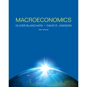
Check here to see more details.
The theory for the long run is driven by the classical theory and generally accepted by the main-stream economics. Post Keynesians, however, want to apply Keynes’ theories in his General Theory also for the long run. Mankiw, the neo-liberal/neo-classical advisor to G. W. Bush, put as follows:
General Theory is an obscure book. We are in a much better position than Keynes was to figure out how the economy works. Classical economics is right in the long run. Moreover, economists today are more interested in the long-run equilibrium. (Mankiw, 1992: 560-61)
Factors that determine Long Run Economic Growth
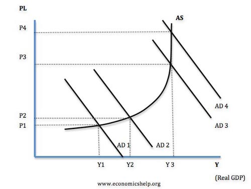
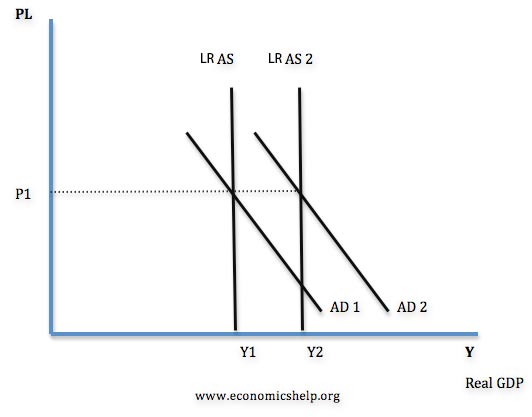
In the long run, economic growth is determined by factors which influence the growth of Long Run Aggregate Supply (LRAS). If there is no increase in LRAS, then a rise in AD will just be inflationary.
This graph shows an increase in LRAS and AD, leading to an increase in economic growth without inflation.
Long Run Aggregate Supply
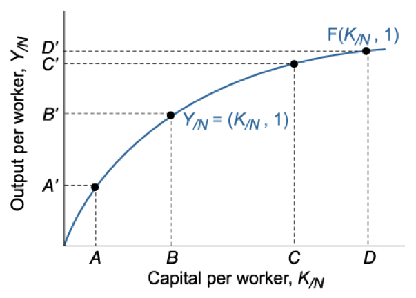
Capital per Worker: Increases in output per worker (Y/N) can come from increases in capital per worker (K/N).
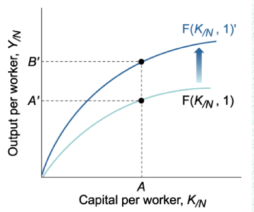
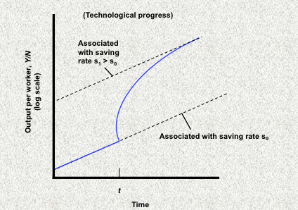
Development of Technology. In the long run development of new technology is a key factor in enabling improved productivity and higher economic growth. An economy that possesses a higher rate of technological progress will perform better than others. Improvements in technology move the production function upwards as shown below.
Saving and Investment
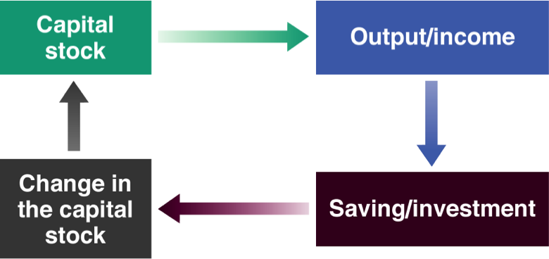
The following “virtuous circle” shows how higher income leads to higher savings and higher investment. This increases the capital stocks and leads via capital per worker to higher output again.
This circle cannot be applied ad infinitum, a fact we show in the next chapter.
The relationships is not necessarily one to one in reality, here the example of China
Long-term Growth Models
In this chapter we describe different models for long-term growth.
Harrod-Domar Model
Assumptions:
(A1) Output is proportional to Capital: Yt = aKt
(A2) Investment ex ante equals Saving: It = St
(A3) Saving proportional to output: St = sYt
(A4) Labor force incases at rate n
(A5) Labor productivity increases at rate m
In equilibrium: g = n + m Growth = Labor force increase + Labor productivity increase
If g < n + m, then we run out of jobs: unemployment
If g > n+ m, then we run out of workers
Main critique:
(A1): in developed economies a is between 0.2 and 0.6, but developing economies capital may be held back.
Solow’s Growth Model
a = Y/K (Output/Capital), S savings, Yt output, At technological progress
Lt rate of population growth,
Kt = It – dKt : Capital is investment minus depreciation_factor * capital
Assumptions:
(A1) Diminishing returns to K for a given state of technology
(A2) Exogenous technological progress, rate: m
(A3) All countries share the same technology
If labor becomes scarce, n < S* a – m
- then wage rates increase and firms will substitute capital for labor, a falls
If labor becomes abundant, n > S* a – m,
- then wage rates decrease, firms will substitute labor for capital, a rises
The steady-state equilibrium implies that further capital per worker does not help increase output per worker. In the very long run this steady state is reached.
The followings are further results:
- The farther away the economy is from its long run equilibrium the faster is the rate of growth of the capital stock and output.
- Rich countries have higher saving (investment) rates relative to population growth than poor countries.
- Permanent differences can only be due to differences in rate of technological progress. If everyone has access to the same technology then growth rates must be the same. Temporary differences are due to transition dynamics.
- Variability of growth rates over time for a given country can be explained by transition dynamics and/or shocks to the parameters.
“Policy pessimism”: - In the (very) long run, growth is driven by technological progress, not by saving rate.
- In the (very) long run, the growth rate of output per worker is zero.
- Differences in per-capita GDP reflect differences in rates of saving and population growth. Before reaching the steady state, the
- Cross-country convergence in growth rates in the (very) long run.
The Golden Rule of Capital
Solow’s model states that the farther away the economy is from its long run equilibrium the faster is the rate of growth of the capital stock and output. This can be translated into the Fixed Investment component of the GDP.
A higher savings rate leads to a period of higher growth boosting technology, which leads to a new, higher path of output per worker.
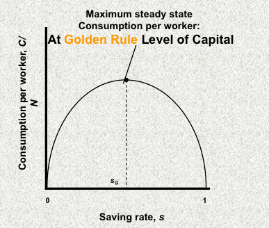
An increase in the savings rate implies lower consumption for some time, but higher consumption later. China follows this model.The level of capital associated with the saving rate that yields the highest level of consumption in steady is the golden-rule level of capital.
Blanchard explains the longer period of slower US growth with the low savings rate.
He maintains that the golden-rule level of capital is 50%.
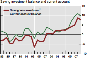
Savings Rate vs. Investment and the U.S. Savings Gap
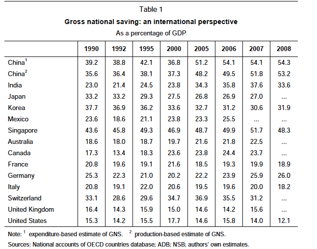
Source BIS
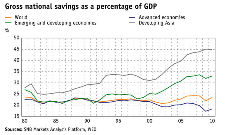
Savings Rate Emerging vs. Advanced Economies 1980-2011, source1
A high savings rate leads also to a high investment share of GDP.
In the aftermath of 1998 Asia crisis, the concerned economies started to accumulate reserves to be able to survive a such crisis better. Federal Reserve Chairman Ben Bernanke said “…the very substantial shift in the current accounts of developing and emerging-market nations … transformed these countries from net borrowers on international capital markets to large net lenders.”
((Taylor, John B. 2009. Competing Explanations: A Global Savings Glut. pp. 6-7.)) ((Bernanke, Ben S. 2005.)) The Global Savings Glut and the U.S. Current Account Deficit. Remarks at the Sandridge Lecture, Virginia Association of Economists, Richmond, Virginia. 10 March 2005.))
Others said that 2000 and 2010, the US savings gap, and the surge in savings in the rest of the world effectively cancelled one another out.2
Endogenous Growth Models
Assumptions (“Policy optimism”, governments can actively influence progress and output) :
(A1) Diminishing returns to capital for given state of technology
(A2) Technological progress (productivity gains) arises from within the economic system
(A3) Countries use different technologies, owing to costly technology transfer
Implications
- In the long run, growth is driven by technological progress, which is endogenously determined
- Differences in per-capita GDP can reflect differences in technology
- Cross-country divergence in levels and growth rates of per-capita GDP
Solow Growth Accounting
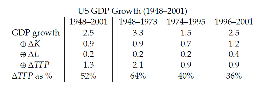
Growth models present a theoretical framework for understanding the sources of economic growth, and the consequences for long-run growth of changes in the economic environment and in economic policy. Often, however, we wish to examine economic growth in a more agnostic framework—without necessarily being bound to pre-adopt the conclusions of any given model. In order to conduct such analysis, economists have built up an alternative framework called growth accounting to obtain a factual perspective on the sources of economic growth.
Further production factors that influence long-term growth
Levels of infrastructure.
Investment in roads, transport and communication can help firms reduce costs and expand production. Without necessary infrastructure it can be difficult for firms to be competitive in the international markets. This lack of infrastructure is often a factor holding back some developing economies.
Human Capital.
Human capital is the productivity of workers. This will be determined by levels of education, training and motivation. Increased labour productivity can help firms take on more sophisticated production processes and become more efficient.
Total Factor Productivity (TFP):
It is the result of an invention, the adoption of an existing technology; a managerial innovation; the re-allocation of factors across sectors and firms
The world bank provides a very nice presentation on the different growth models:
[gview file=”https://snbchf.com/wp-content/uploads/2012/10/Growth-Models.pdf”]
Further Bibliography
Harrod, Roy F. (Mar. 1939). “An Essay in Dynamic Theory”. The Economic Journal 49 (193): 14–33.
Domar, Evsey (April 1946). “Capital Expansion, Rate of Growth, and Employment”. Econometrica 14 (2): 137–47.
Mankiw, N.G.(1992), “The Reincarnation of Keynesian Economics”, European Economic Review, 36. Quote taken from Davidson, (1994).
Ricardo, D. (1817), On the Principles of Political Economy and Taxation. (The first economist to formulate the axiom of perfect certainty in economics.)
Robert Merton Solow: A Contribution to the Theory of Economic Growth. In: Quarterly Journal of Economics, Band 70, 1956, S. 65–94 (doi:10.2307/1884513).
- Danthine, Jean-Pierre. 2012. ‘A world of low interest rates’ Swiss National Bank. Online, March 2012 [↩]
- Taylor, John B. 2009. Competing Explanations: A Global Savings Glut. pp. 6-7. [↩]


